What is a good level of forecast accuracy?
The most common question we get from customers, consultants, and other business experts is, “What would you consider a good level of forecast accuracy in our business?” The thing to consider, however, is that incorporating accurate forecasting into your inventory management strategy is more complex than aiming for a number.
In any consumer goods value chain context, forecasting is always a means to an end, not the end itself. A forecast is relevant only in its capacity to help us achieve other goals, such as improved on-shelf availability, reduced food waste, or more effective assortments.
While forecasting is an integral part of any planning activity, it still represents only one cogwheel in the planning machinery, meaning that other factors may significantly impact the outcome. Accurate forecasting is crucial most of the time, but occasionally, other factors will substantially impact getting the desired results.
We aren’t saying that you should stop measuring forecast accuracy altogether. Forecast accuracy measurement plays an essential role when doing root cause analysis of supply chain problems, and detecting systematic forecast accuracy changes early on can help identify relevant changes in customer demand patterns.
To get truly valuable insights out of forecasts, you need to understand the following:
- The role of demand forecasting in attaining business results. Demand forecast accuracy is crucial when managing short-shelf-life products such as fresh food. However, for other products, such as slow-movers with long shelf lives, other parts of your planning process may have a more significant impact on your business results. Can you differentiate between which products and situations need high forecast accuracy to drive business results and which do not?
- Which factors affect your attainable forecast accuracy. Demand forecasts are inherently uncertain — that’s why we call them forecasts, not plans. Demand forecasting is easier in some circumstances than in others. Do you know when you can rely more heavily on forecasting and when to set up your operations to have a higher tolerance for forecast errors?
- How to assess forecast quality. Forecast metrics can be used for monitoring performance and detecting anomalies — but how can you tell whether your forecasts are already of high quality or whether there is still significant room for improvement in your forecast accuracy?
- How the main forecast accuracy metrics work. When measuring forecast accuracy, the same data set can lead to different forecasts depending on the chosen metric and how you conduct the calculations. Different metrics measure different things and, therefore, can give conflicting views as to the quality of the forecast.
- How to monitor forecast accuracy. No forecast metric is universally better than another. Do you know which forecast accuracy formula to use and how?
By the end of this guide, you’ll understand these foundational elements of forecast accuracy and how to use them to optimize inventory management.

1. The role of demand forecasting in attaining business results
Good demand forecasts reduce uncertainty. In retail distribution and store replenishment, good forecasting will help you boost product availability, reduce safety stock, increase margins, minimize waste, and reduce the need for clearance sales. Further up the supply chain, good forecasting allows manufacturers to secure the availability of relevant raw and packaging materials and operate their production with lower capacity, time, and inventory buffers.
Forecasts are obviously important. For example, advanced machine learning (ML) with demand sensing gives insights into the complex relationships between demand and influencing factors. On the other hand, demand forecasts will always be inaccurate to some degree, and the planning process must accommodate this with a probabilistic understanding of demand using modeled demand distribution in all planning activities.
In some cases, mitigating the effect of forecast errors may be more cost-effective than investing in increasing forecast accuracy. In inventory management, the cost of a moderate increase in safety stock for a long lifecycle and long shelf-life product may be quite reasonable, especially when compared to the time it takes a demand planner to fine-tune forecasting models or make manual changes to the demand forecast. If that wasn’t enough, and if the remaining forecast error is caused by random variation in demand, any attempt to increase forecast accuracy will be fruitless.
Other factors may significantly impact business results more than perfecting your demand forecast. See Figure 1 for an example of forecasting in grocery store replenishment planning. Although the forecast accuracy for the example product and store is quite good, there is still systemic waste due to product spoilage. When digging deeper into the matter, it becomes clear that the main culprit behind the excessive waste is the product’s presentation stock, or the amount needed to keep its shelf space sufficiently full to maintain an attractive display. By assigning less space to the product (Figure 2), inventory levels can be pushed down, allowing for 100% availability with no waste — all without changing the forecast.
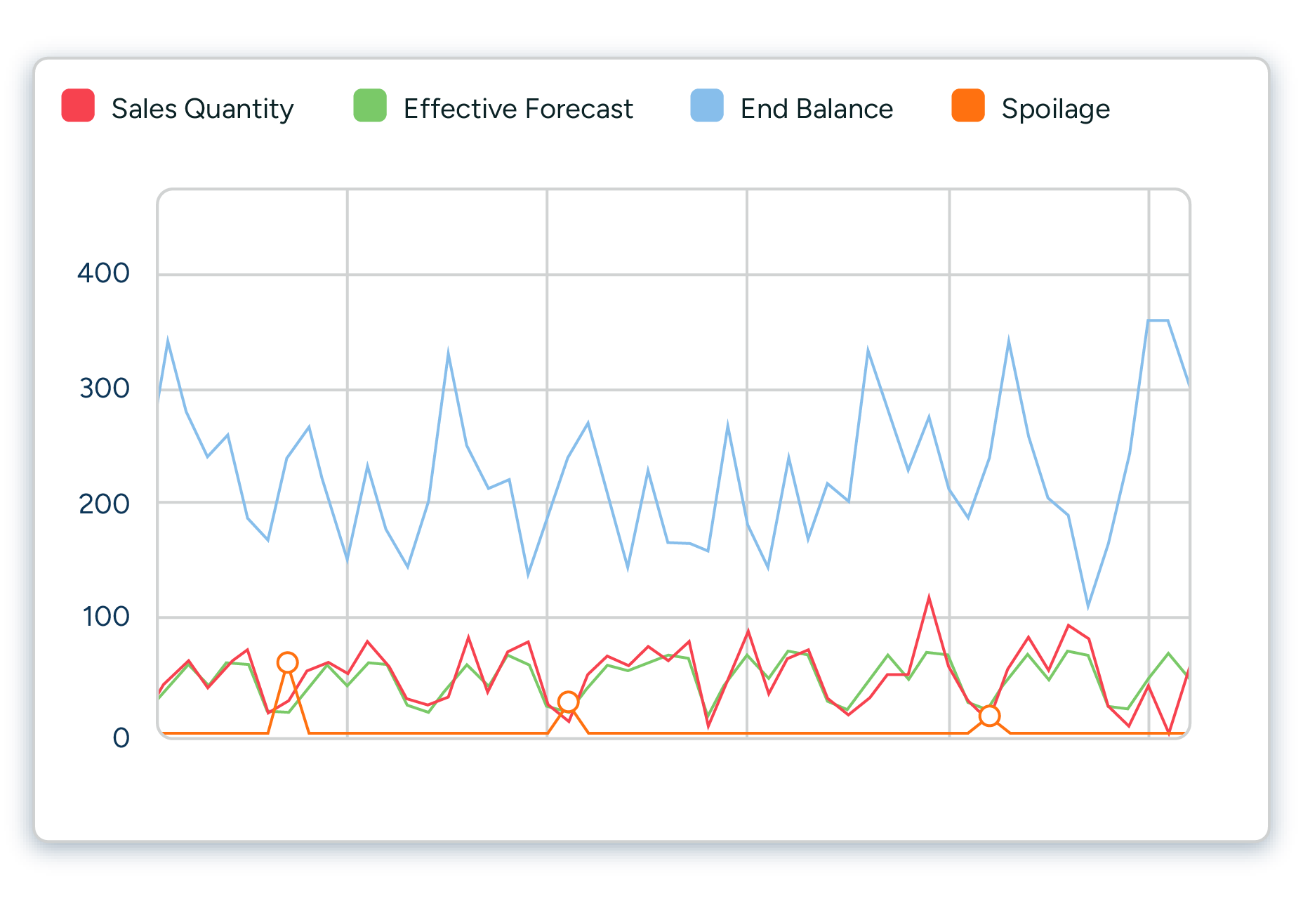
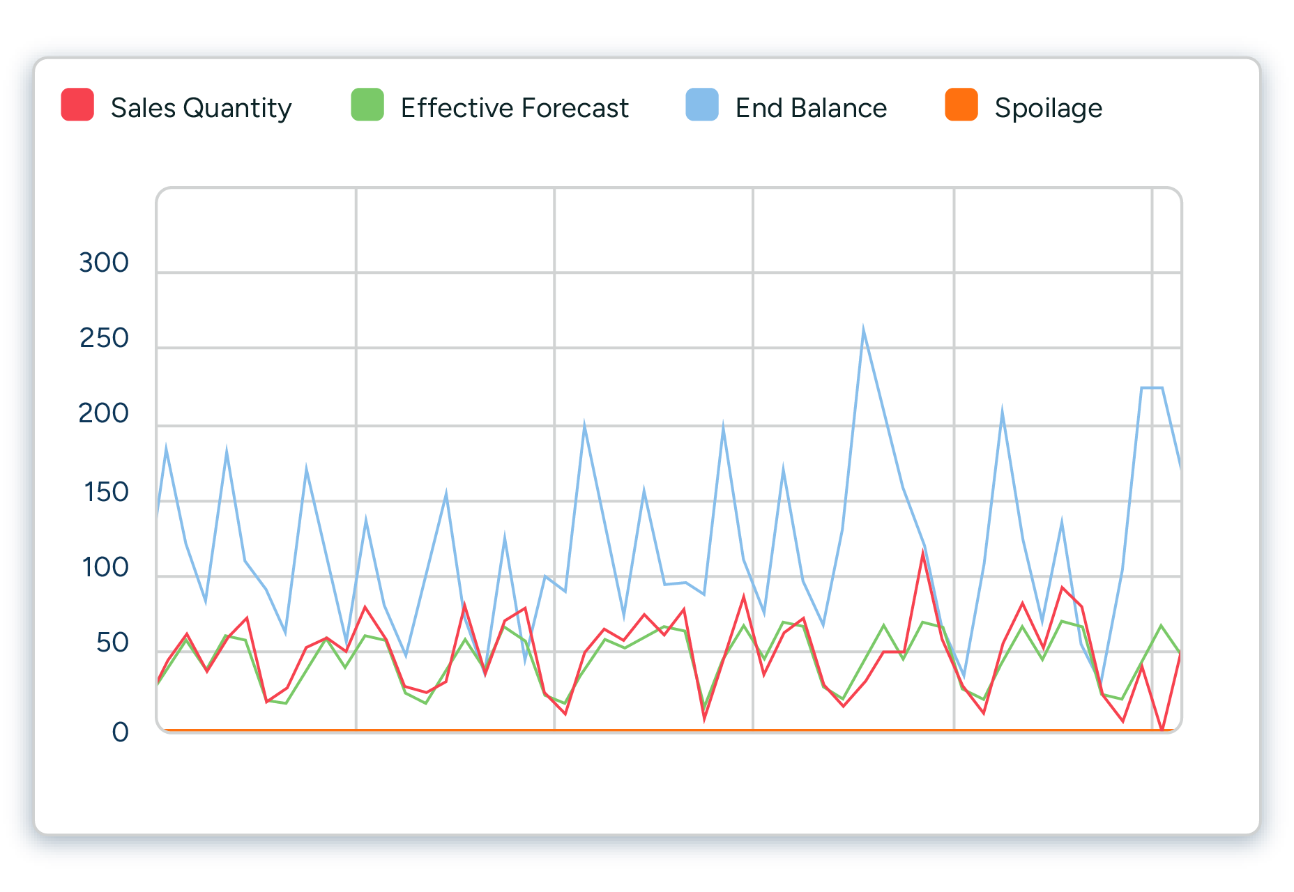
Forecasts can only deliver results if the other parts of the planning process are equally effective. In some situations – like fresh food retail – forecasting is crucial. It makes business sense to invest in tools that capture all demand-influencing factors accurately, such as weather, promotions, and cannibalization, which may diminish demand for substitute items. (You can read more about fresh food forecasting and replenishment in our guide.)
However, all this work will not pay off if batch sizes are too large or there is excessive presentation stock.
This, of course, applies to any planning process. Suppose you only focus on forecasts and do not spend time on optimizing the other elements impacting your business results, like safety stocks, supplier reliability, lead times, batch sizes, or planning cycles. In that case, you will reach a point where additional improvements in forecast accuracy will only marginally improve the actual business results.
Forecast accuracy is only the beginning
In recent years, we have seen an increasing trend of retailers holding forecast competitions to choose between planning software providers. In a forecast competition, all vendors get the same data from a retailer, which they then load into their planning tools to show what level of forecast accuracy their system can provide. May the best forecast win!
We are in favor of customers getting hands-on experience with the software and an opportunity to test its capabilities before making a purchase decision.
There is, however, also reason for caution when setting up forecast competitions. In some cases, we have been forced to choose between the forecast getting us the best score for the selected forecast accuracy metric or presenting the forecast that we know would be the best fit for its intended use. How can this happen?
When discussing forecasting metrics such as WAPE (Weighted Absolute Percentage Error) or MSE (Mean Squared Error), it’s essential to understand their context within the process used. WAPE measures the accuracy of a forecast by comparing the absolute errors to the actual values, giving more weight to larger values. MSE, on the other hand, calculates the average of the squared differences between predicted and real values, emphasizing larger errors due to the squaring effect.
A problem related to many forecasting metrics (like WAPE or MSE) is that they are not linked to the process they’re used in. For example, if forecast accuracy as measured by 1-WAPE is 48%, is that a good or a bad result? If it’s a bad result, does it matter? The following figures demonstrate this example:
Say you have a product-location with average daily sales of 0.23 pcs. Forecast bias is acceptable at 101%, while forecast accuracy (1-WAPE) is only 15%.
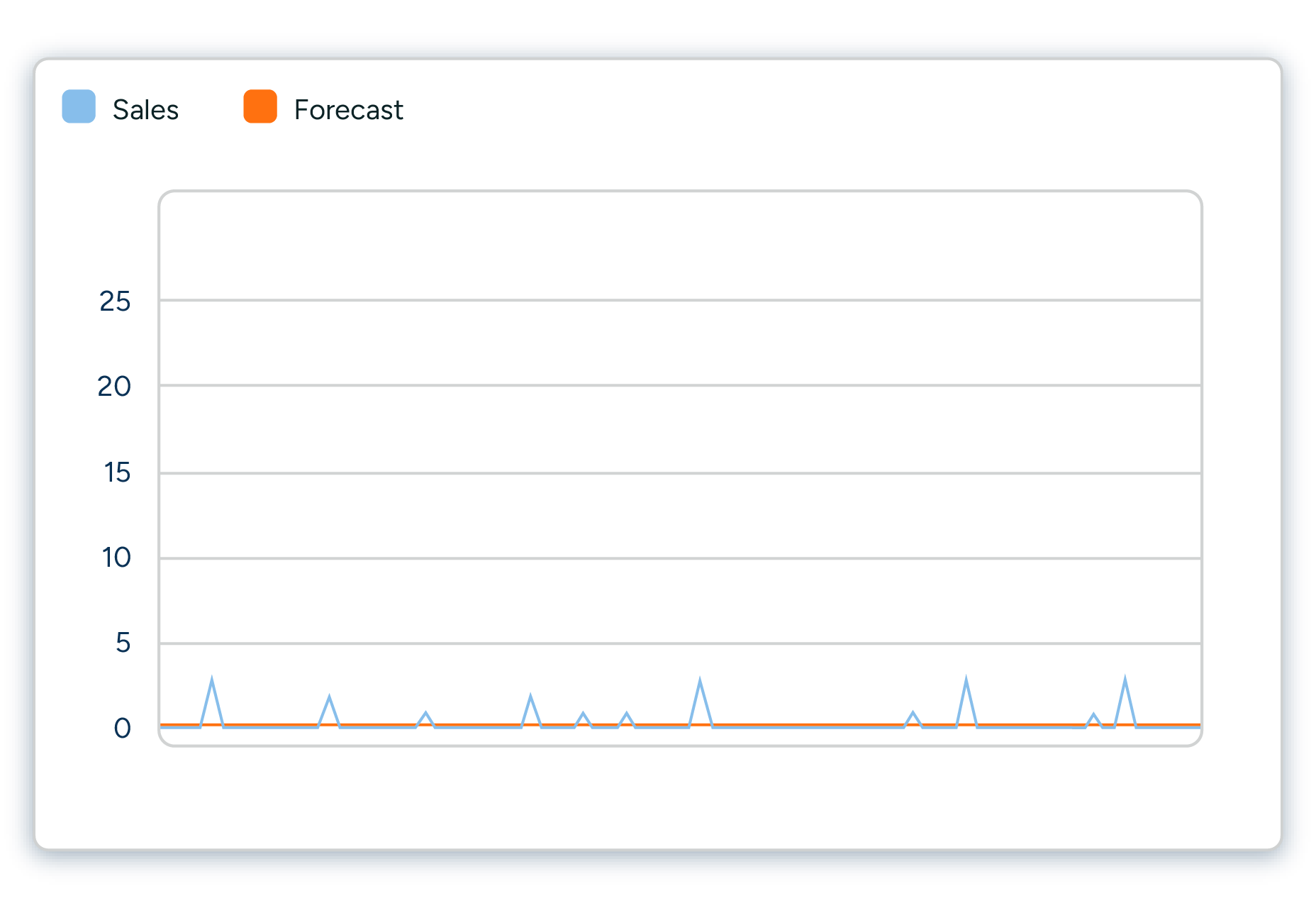
But remember that you also need to consider the use case – replenishment for this product location is driven by batch size and other replenishment parameters. The not-so-good forecast accuracy of 15% is acceptable for direct replenishment needs since it does not directly affect the ordering frequency or accuracy.
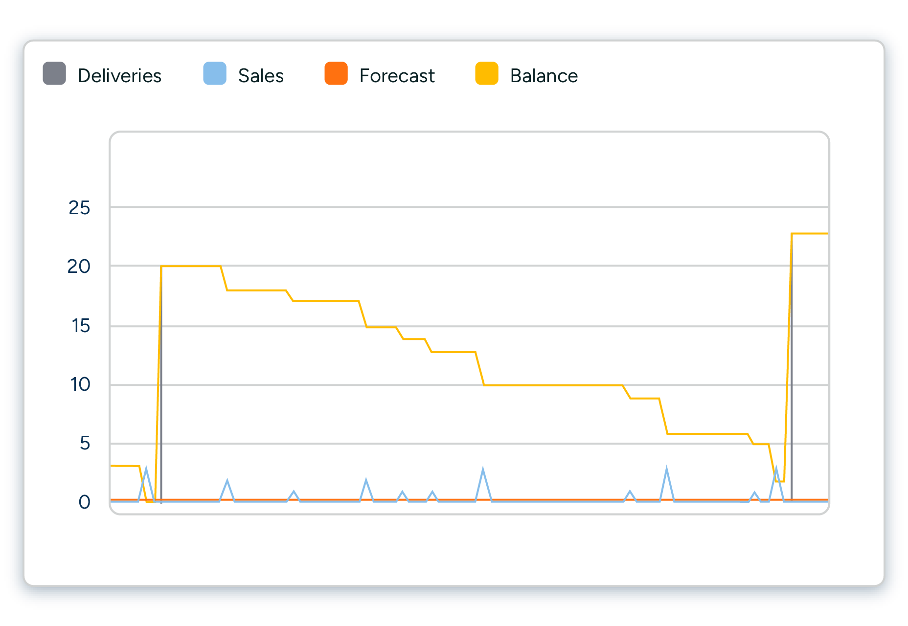
For this situation, you need forecast metrics that can be tied to replenishment ordering as a specific use case.
Forecast error and bias in batches serve this purpose well. The calculation formulas are as follows:
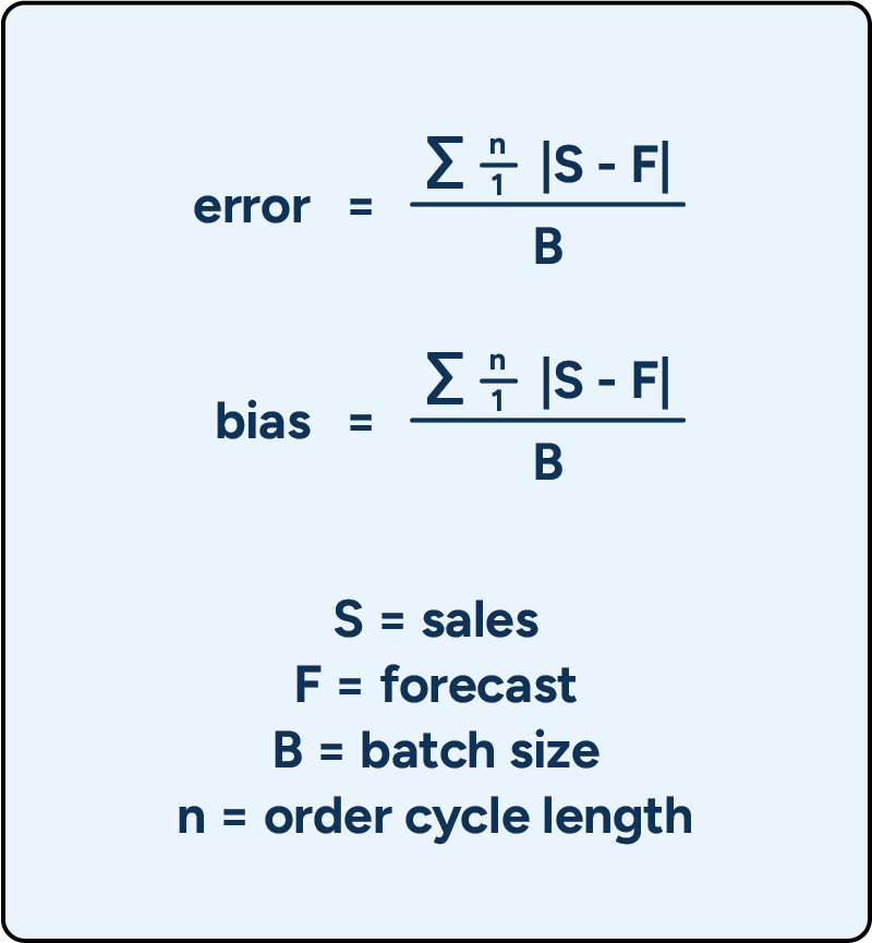
These metrics reveal whether any forecast error or bias during replenishment order calculation was large enough to cause a different order quantity than an order with 100% forecast accuracy. These metrics are computed as an average over the entire time horizon, which gives us many data points, makes the metrics reliable, and automatically considers any parameter changes to delivery schedules or batch sizes.
For example, a product with an average forecast error in batches over the order cycle of 0.85 indicates that, on average, we are nearly one batch off. This discrepancy drives incorrect replenishment decisions, which is evident through frequent stockouts. (See Figure 5 below.)
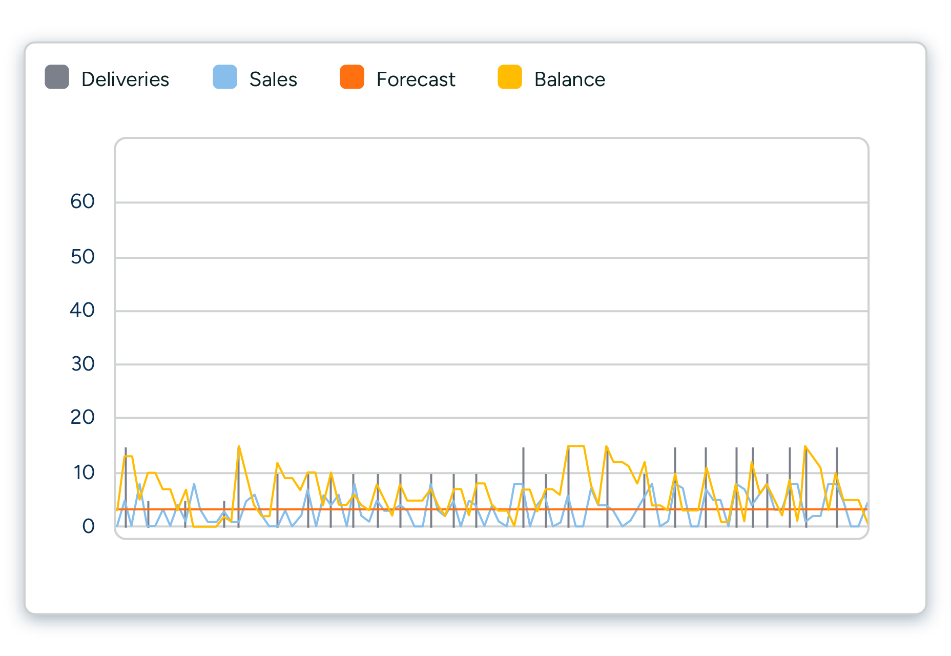
In contrast, consider an example product with the same sales rate and delivery schedules but a batch size of 50 instead of five. The average forecast error in batches over the order cycle is 0.085, indicating that any potential suboptimal ordering is not driven by forecast error. (See Figure 6 below.)
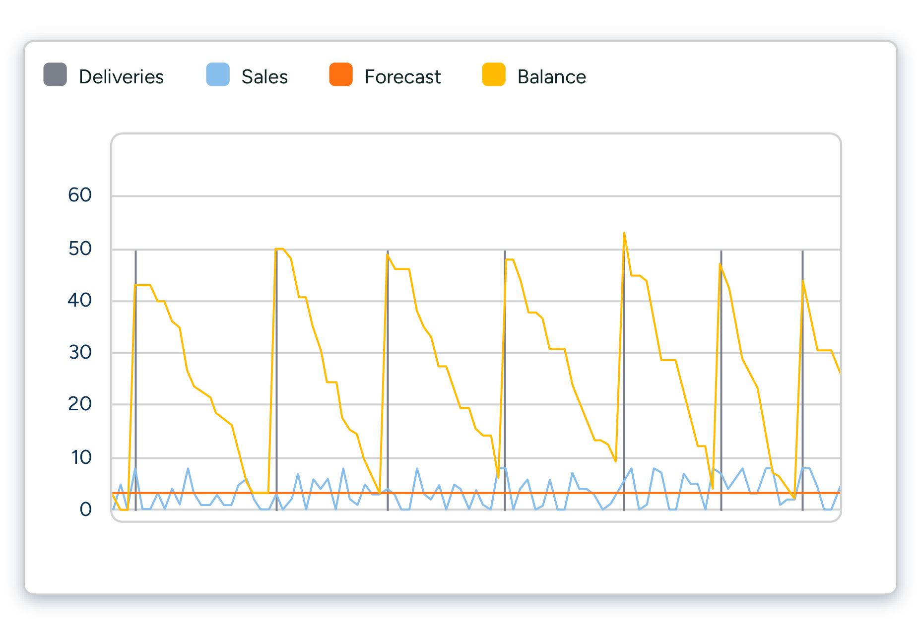
In this situation, it’s best to aim for a forecast accuracy threshold of “good enough” and focus all forecast-related efforts on the right products. For example, a cycle forecast error in batches less than 0.25 means ordering decisions are not affected by forecast inaccuracy. Don’t focus your forecasting efforts on these products.
On the other hand, a cycle forecast error in batches greater than 1 means your forecast inaccuracies are actively distorting optimal order quantities. Focus your forecasting efforts on these products, and do it in business impact priority order, starting from products with the highest cycle forecast error in batches.
The examples also show that products don’t need to be categorized because these metrics are scale-agnostic. The effect on replenishment doesn’t change regardless of the level of demand. The same isn’t true for 1-WAPE, though. For some products (like very slow-moving products with intermittent demand), the forecast accuracy of 10% might be a good figure; for others, it’s horrible.
The most frustrating aspect of comparing forecasts is the lack of a universal benchmark or standard that accurately reflects the unique operational realities and challenges of different products and industries.
By manipulating the forecast formula to underestimate demand consistently, the day-level forecast accuracy for slow-moving products can often be significantly increased. However, at the same time, this would introduce a significant bias to the forecast with the potential of considerably hurting supply planning in a situation where store forecasts form the basis for the distribution center forecast. And there would be no positive impact on store replenishment.
So, for our slow-moving example product, the forecast giving us a better score for the selected forecast accuracy metric is less fit for driving replenishment to the stores and distribution centers than the forecast attaining a worse forecast accuracy score.
2. What factors affect your attainable forecast accuracy
Several factors impact the level of forecast accuracy that can realistically be attained. This is one of the reasons it’s so challenging to compare forecast accuracy between companies or even between products within the same company. There are a few basic rules of thumb, though, to understanding which factors impact attainable forecast accuracy:
Forecasts are more accurate when sales volumes are high
It is generally easier to attain higher forecast accuracy for large sales volumes. If a store only sells one or two units of an item per day, even a random one-unit variation in sales will result in a significant percentage forecast error. By the same token, large volumes lend themselves to leveling out random variation.
For example, if you already sell hundreds of 12 oz. cans of Coke from your store on a daily basis, a busload of tourists stopping by that store to each buy a can of Coke will not significantly impact forecast accuracy. However, suppose the same tourists receive a mouthwatering recommendation for a beer-seasoned mustard that the store carries. In that case, their purchases will correspond to a month’s worth of demand and most likely leave the shelves all cleaned out.
Forecast accuracy improves with the level of aggregation
When aggregating over SKUs or over time, we see the same effect of larger volumes dampening the impact of random variation. This means that forecast accuracy measured on a product-group level or for a chain of stores is higher than when looking at individual SKUs in specific stores. For the same reasons, forecast accuracy is usually significantly higher when measured monthly or weekly than daily.
Short-term forecasts are more accurate than long-term forecasts
A longer forecasting horizon significantly increases the chance of unanticipated changes impacting future demand. A simple example is weather-dependent demand. If we need to decide what quantities of summer clothes to buy or produce half a year or even longer in advance, there is currently no way of knowing what the weather will actually be like when summer arrives. On the other hand, if we manage the replenishment of ice cream to grocery stores, we can use short-term weather forecasts when planning how much ice cream to ship to each store.
Forecasting is easier with steady businesses
Attaining good forecast accuracy for mature products with constant demand is always easier than for new products – that’s why forecasting in fast fashion is more complex than in grocery. In grocery supply chains, retailers following a year-round, low-price model find forecasting easier than competitors that rely heavily on promotions or frequent assortment changes.
Now that we have established that there cannot be any universal benchmarks for when forecast accuracy can be considered satisfactory or unsatisfactory, how do we identify the potential for improvement in forecast accuracy?
3. How to assess forecast quality
The first step is assessing your business results and the role forecasting plays in attaining them. If forecasting is the main culprit in explaining disappointing business results, you must examine whether your forecasting performance is satisfactory.
Do your forecasts accurately capture systemic variation in demand?
There are usually many types of somewhat systemic demand variation. There may be seasonality, such as demand for tea increasing in the winter, or trends, such as an ongoing increase in demand for organic food, that can be detected by examining past sales data. In addition, many products have distinct weekday-related variations in demand, especially at the store and product levels. A good forecasting system using sophisticated AI algorithms should be able to identify these kinds of systemic patterns without manual intervention.
Do your forecasts accurately capture the impact of business decisions known beforehand?
Internal business decisions, such as promotions and price and assortment changes, directly impact demand. If these planned changes are not reflected in your forecast, you need to fix your planning process before you can start addressing forecast accuracy. The next step is to examine how you forecast, for example, the impact of promotions. Are you already taking advantage of all available data in your forecasting formula, such as promotion type, marketing activities, price discounts, in-store displays, etc., or could you improve accuracy through more sophisticated forecasting?
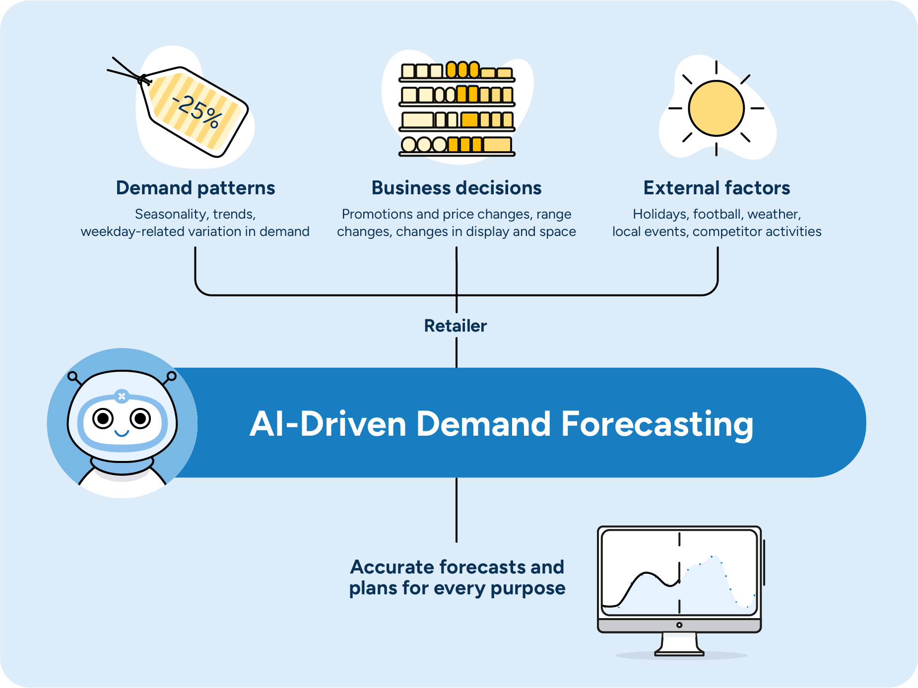
In addition to your organization’s own business decisions, there are external factors that have an impact on demand. Some of these are known well in advance, such as holidays or local festivals. Forecasting can be highly automated for recurring events, such as Valentine’s Day, for which past data is available. Some external factors naturally take us by surprise, such as a specific product taking off on social media. Even when information becomes available only after important business decisions have been made, it is essential to use that information to cleanse the data used for forecasting to avoid errors in future forecasts.
Does your forecast accuracy behave predictably?
It is often more important to understand in which situations and for which products forecasts can be expected to be good or bad rather than to pour vast resources into perfecting forecasts that are by nature unreliable. Understanding when forecast accuracy is likely to be low makes it possible to do a risk analysis of the consequences of over- and under-forecasting and make business decisions accordingly.
A good example of this is a fast-moving consumer goods (FMCG) manufacturer we have worked with, who has a process for identifying potential “stars” in their portfolio of new products. “Star” products have the potential to break the bank — but they’re rare and seen only a couple of times each year. As the products have limited shelf life, the manufacturer does not want to risk potentially inflated forecasts driving up inventory “just in case.” Instead, they ensure they have production capacity, raw materials, and packaging supplies to deal with a scenario where the original forecast is too low.
The need for predictable forecast behavior is also why we apply extreme care with machine learning algorithms. For example, when testing promotion data, we might discard one approach that is, on average, slightly more accurate than others but significantly less robust and more difficult for the average demand planner to understand. Occasional extreme forecast errors can be detrimental to your performance when the planning process has been set up to tolerate a certain level of uncertainty. These errors also reduce the demand planners’ confidence in the forecast calculations, significantly hurting efficiency.
Suppose demand changes in ways that cannot be explained, or demand is affected by factors for which information is not available early enough to impact business decisions. In that case, you must find ways to make the process less dependent on forecast accuracy.
We have already mentioned that weather is one external factor that impacts demand. In the short term, weather forecasts can be used to drive replenishment to stores (you can read more about how to use machine learning to benefit from weather data in your forecasting here). However, long-term weather forecasts are still too uncertain to provide value in demand planning, which must be done months before sales.
In very weather-dependent businesses, such as winter sports gear, it’s essential to make strategically sound decisions about what inventory levels to go for. For high-margin items, the business impact of losing sales due to stock-outs is usually worse than the impact of needing to resort to clearance sales to get rid of excess stock, which is why it may make sense to plan in accordance with favorable weather. For low-margin items, rebates may quickly turn products unprofitable, which is why having a more cautious inventory plan may be wiser.
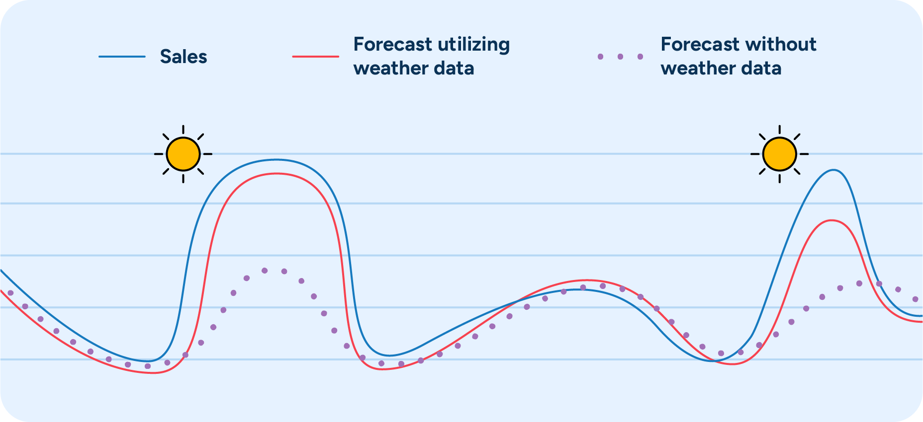
In any case, setting up your operations so that final decisions on where to position stock are made as late as possible allows time to collect more information and improve forecast accuracy. In practice, this can mean holding back a proportion of inventory at your distribution centers to be allocated to the regions with the most favorable conditions and the best chance of selling the goods at full price. (You can read more about managing seasonal products here.)
4. How the main forecast accuracy metrics work
Depending on the chosen metric, level of aggregation, and forecasting horizon, you can get significantly different forecast accuracy results for the same data set. To analyze forecasts and track the development of forecast accuracy over time, you need to understand the essential characteristics of commonly used forecast accuracy metrics.
Most are variations of the following three: forecast bias, mean average deviation (MAD), and mean average percentage error (MAPE). We’ll take a closer look at these next — but don’t let the simple appearance of these metrics fool you. After explaining the basics, we’ll delve into the intricacies of calculating these metrics in practice and show how simple and completely justifiable changes in your calculation logic can radically alter forecast accuracy results.
Forecast bias is the difference between the forecast and actual sales. If the forecast overestimates sales, the forecast bias is considered positive. If the forecast underestimates sales, the forecast bias is considered negative. If you want to examine bias as a percentage of sales, divide the total forecast by total sales – results of more than 100% mean that you are over-forecasting and results below 100% that you are under-forecasting.

In many cases, knowing whether demand is systemically over- or under-estimated is helpful. For example, a slight forecast bias may not have a notable effect on a single store’s replenishment. Still, if this type of systematic error concerns many stores, it can lead to over- or under-supply at the central warehouse or distribution centers.
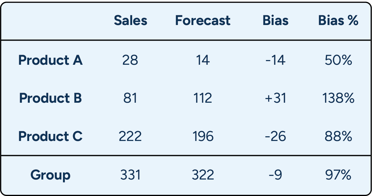
A word of caution: When looking at aggregations over several products or long periods, the forecast bias metric can’t provide much information on the quality of the detailed forecasts. The bias metric only tells you whether the overall forecast was good and can easily disguise substantial errors. You can find an example of this in Table 1 below.
This example shows weekly sales and forecasts for three items. Although the biases for each product are quite large, the group-level bias calculated by comparing total sales to the total forecast for all three products is minimal. In other words, on an aggregated level, the forecast looks great, and the bias is close to the target of 100%.
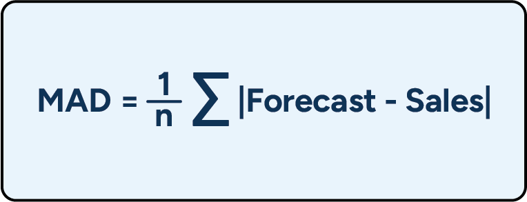
Mean absolute deviation (MAD) is another commonly used forecasting metric. This metric shows how large an error, on average, you have in your forecast. However, because the MAD metric gives you the average error in units, it is not very useful for comparisons.
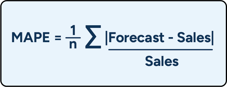
Mean absolute percentage error (MAPE) is akin to the MAD metric but expresses the forecast error in relation to sales volume. Essentially, it tells you how many percentage points your forecasts are off, on average. This is probably the single most used forecasting metric in demand planning.
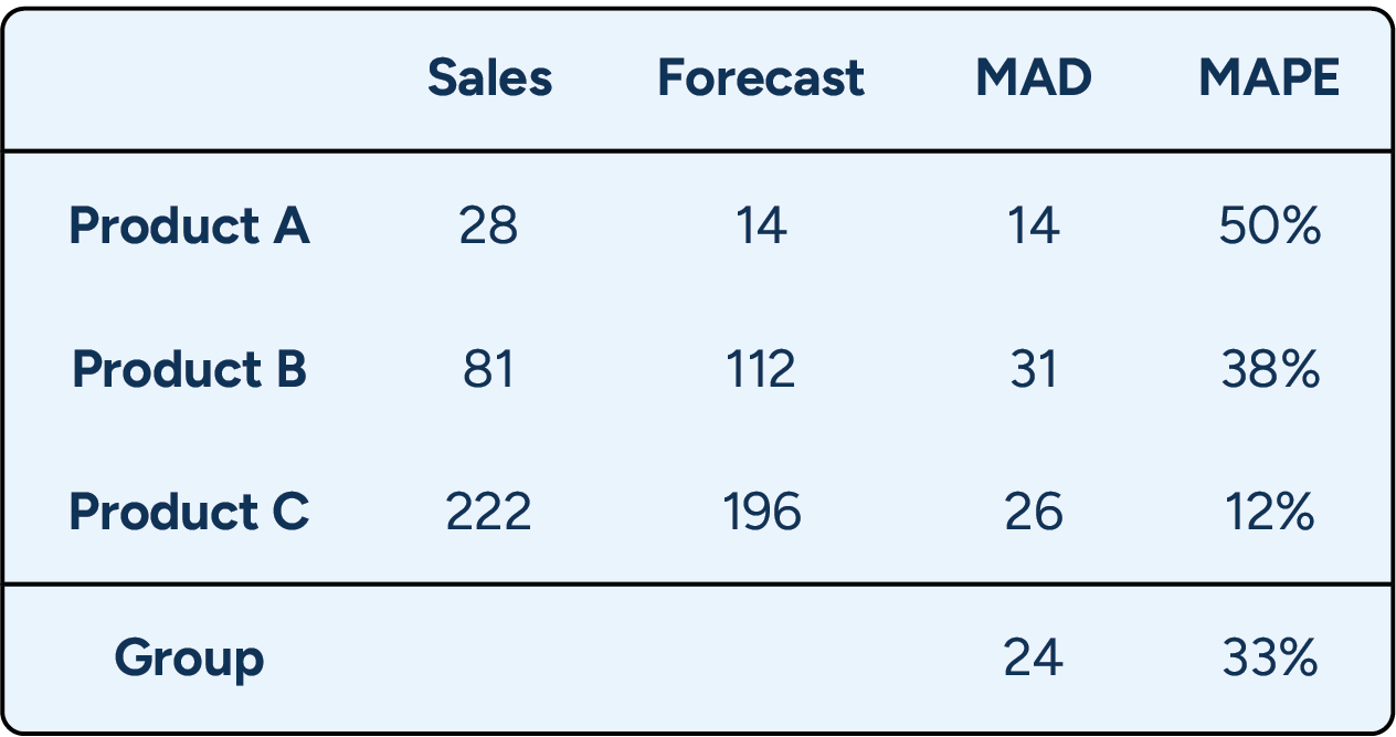
MAPE calculations give equal weight to all items, whether products or periods, so they quickly produce substantial error percentages if you include many slow-movers in the data set, as relative errors amongst slow-movers can appear rather large even when the absolute errors are not (see Table 1 for an example of this). In fact, a typical problem when using the MAPE metric for slow movers on the day level is sales being zero, making it impossible to calculate a MAPE score.
Measuring forecast accuracy is not only about selecting the right metric (or metrics). There are a few more things to consider when deciding how you should calculate your forecast accuracy:
Measuring accuracy or error may seem like self-explanatory concepts, but some very smart people get confused over terminology. Despite the name, forecast bias measures accuracy: the target level is 1 or 100%, and the number +/- is the deviation. MAD and MAPE, however, measure forecast error: the target level is 0 or 0%, and larger numbers indicate larger errors.
Aggregating data or aggregating metrics is one of the most significant factors affecting your forecast accuracy formula’s results. As discussed earlier, forecast accuracies are typically better when viewed on the aggregated level. However, when measuring forecast accuracy at aggregate levels, you must also be careful about how you perform the calculations. As we will demonstrate below, it can make a huge difference whether you apply the metrics to aggregated data or calculate averages of the detailed metrics.
The example (see Table 3) shows three products, their sales and forecasts from a single week, and their respective MAPEs. The bottom row shows sales, forecasts, and the MAPE calculated at a product group level based on the aggregated numbers. Using this method, we get a group-level MAPE of 3%. However, as we saw in Table 2, if one first calculates the product-level MAPE metrics and then calculates a group-level average, we arrive at a group-level MAPE of 33%.
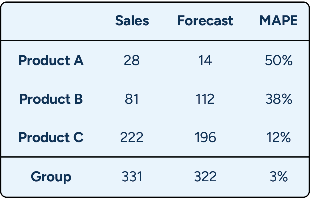
Which number is correct? The answer is that both are, but they should be used in different situations and never be compared to one another.
For example, when assessing forecast quality from a store replenishment perspective, one could easily argue that the low forecast error of 3% on the aggregated level would, in this case, be quite misleading. However, suppose the forecast is used for business decisions on a more aggregated level, such as planning picking resources at a distribution center. In that case, the lower forecast error of 3% may be perfectly relevant.
The same dynamics are at play when aggregating over periods of time. The data in the previous examples were on a weekly level. Still, the results would look quite different if we calculated the MAPE for each weekday separately and then took the average of those metrics. In the first example (Table 2), the product-level MAPE scores based on weekly data were between 12% and 50%. However, the product-level averages calculated based on the day-level MAPE scores vary between 23% and 71% (see Table 4). By calculating the average of these latter MAPEs, we get a third suggestion for the error across the group of products: 54%. This score is again quite different from the 33% we got when calculating MAPE based on week and product level data and the 3% we got when calculating it based on week and product-group level data.
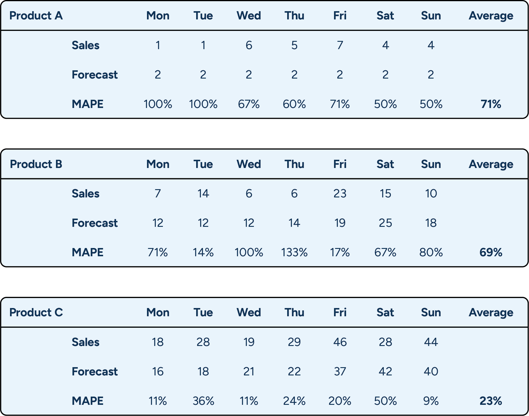
Which metric is the most relevant? If these are forecasts for a manufacturer that applies weekly or longer planning cycles, measuring accuracy on the week level makes sense. But if we are dealing with a grocery store receiving six deliveries a week and demonstrating a clear weekday-related pattern in sales, keeping track of daily forecast accuracy is much more critical, especially if the items in question have a short shelf-life.
Arithmetic average or weighted average
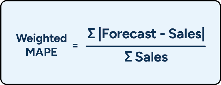
One could argue that an error of 54% does not give the right picture of what is happening in our example. After all, Product C represents over two-thirds of total sales, and its forecast error is much smaller than for the low-volume products. Shouldn’t the forecast metric somehow reflect the importance of the different products? This can be resolved by weighting the forecast error by sales, as we have done for the MAPE metric in Table 5 below. The resulting metric is called the volume-weighted MAPE or MAD/mean ratio.
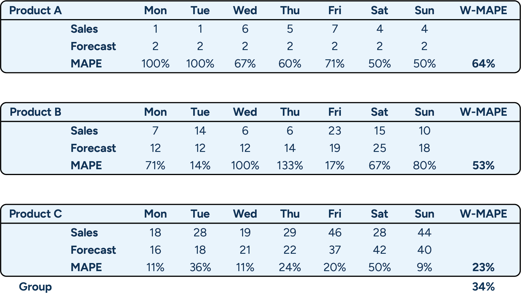
As you see in Table 5, the product-level volume-weighted MAPE results are different from our earlier MAPE results. This is because the MAPE for each day is weighted by the sales for that day. The underlying logic here is that if you only sell one unit a day, an error of 100% is not as bad as when you sold 10 units and suffered the same error. On the group level, the volume-weighted MAPE is now much smaller, demonstrating the impact of placing more importance on the more stable high-volume product.
Choosing between arithmetic and weighted averages is a matter of judgment and preference. On the one hand, it makes sense to give more weight to products with higher sales, but on the other hand, you may lose sight of underperforming slow movers that way.
The final or earlier versions of the forecast
The further into the future you forecast, the less accurate it will be. Typically, forecasts are calculated several months into the future and then updated weekly.
So, for a given week, you usually calculate multiple forecasts over time, meaning you have several different forecasts with different time lags. The forecasts should get more accurate when you get closer to the week you are forecasting, meaning that your forecast accuracy will look very different depending on which forecast version you use when calculating.
The forecast version used to measure forecast accuracy should match the time lag when important business decisions are made. In retail distribution and inventory management, the relevant lag is usually the lead time for a product. If a supplier delivers with a lead time of 12 weeks, what matters is the forecast quality when the order was created, not the forecast when the products arrived.
5. How to monitor demand forecast accuracy
When assessing forecast accuracy, no metric is universally better than another. It’s all a question of what you want to use the metric for:
- Cycle forecast error and bias in batches connect forecasts to business impact. The other metrics do not tell you that.
- Forecast bias tells you whether you are systematically over- or under-forecasting. The other metrics do not tell you that.
- MAD measures forecast error in units. It can, for example, be used to compare the results of different forecast models applied to the same product. That said, the MAD metric is unsuitable for comparing different data sets.
- MAPE is better for comparisons, as the forecast error is compared to sales. However, since all products are given the same weight, it can provide very high error values when the sample contains many slow movers. Using a volume-weighted MAPE places more importance on the high sellers. The downside is that even very high forecast errors for slow movers can go unnoticed.
The forecast accuracy formula should also match the relevant levels of aggregation and the relevant planning horizon. In Table 6, we present a few examples of different planning processes utilizing forecasts and typical levels of aggregation over products and time, as well as the time spans associated with those planning tasks.
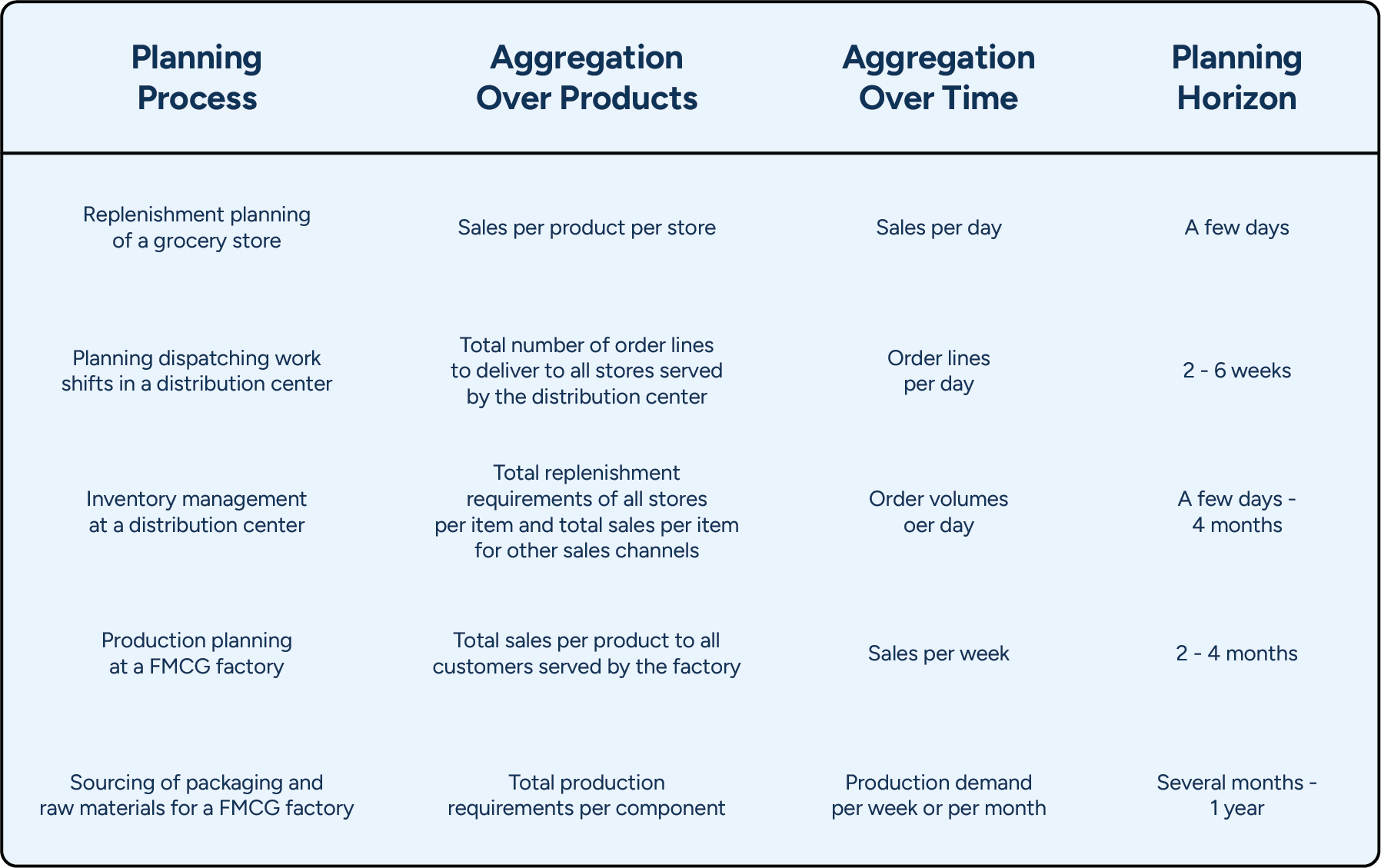
To make things even more complicated, the same forecast is often used for several different purposes, meaning that several metrics with varying levels of aggregation and different time spans are commonly required.
A good example is store replenishment and inventory management at the supplying distribution center. We recommend translating the forecast that drives store replenishment into projected store orders to drive inventory management at the distribution center (DC). That way, changes in the store’s inventory parameters, replenishment schedules, and planned changes in stock positions (to prepare for a promotion or in association with a product launch) are immediately reflected in the DC’s order forecast.
This means that store forecasts must be sufficiently accurate several weeks (or months) ahead. However, the requirements for the store forecasts and the DC forecast are not the same. The store-level forecast needs to be accurate at the store and product levels, whereas the DC-level forecast needs to be accurate for the full order volume per product and all stores.
On the DC level, aggregation typically reduces the forecast error per product. But be careful about systemic bias in the forecasts, as a tendency to over- or under-forecast store demand may become aggravated through aggregation.
The number of forecasts in a retail or supply chain planning context is typically very large, to begin with, and dealing with multiple metrics and formulas means that the number grows even further. This is why you need an exception-based process for monitoring accuracy. Otherwise, your demand planners will either be completely swamped or risk losing valuable demand signals in the averages.
To be able to effectively identify relevant exceptions, try classifying products based on their importance and predictability. This can be done in many ways. However, a simple starting point is to classify products based on sales value (like ABC classification, which reflects economic impact) and sales frequency (like XYZ classification, which tends to correlate with more accurate forecasting). For high sales value and sales frequency AX products, for example, high forecast accuracy is realistic, and the consequences of deviations are quite significant. That’s why the exception threshold should be kept low, and reactions to forecast errors should be quick. For products with low sales frequency, your process must be more tolerant of forecasting errors, and exception thresholds should be set accordingly.
Another good approach, which we recommend using in combination with the above, is singling out products or situations where forecast accuracy is known to be a challenge or of crucial importance. A typical example is fresh or other short-shelf-life products, which should be monitored very carefully as forecast errors quickly translate into waste or lost sales. Special situations, such as new kinds of promotions or product introductions, can require special attention even when the products have a longer shelf-life.
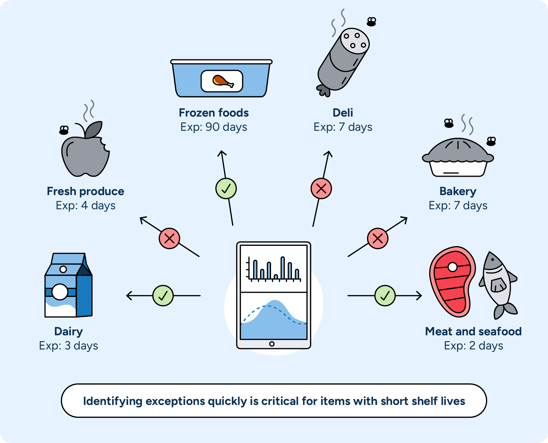
Some forecasting systems on the market look like black boxes to the users: data goes in, forecasts come out. This approach would work fine if forecasts were 100% accurate, but forecasts are never fully reliable. To get value out of monitoring forecast accuracy, you need to be able to react to exceptions. Simply addressing exceptions by manually correcting erroneous forecasts will not help you in the long run, as it does nothing to improve the forecasting process.
Therefore, you need to ensure your forecasting system is 1) transparent enough for your demand planners to understand how any given forecast was formed and 2) allows your demand planners to control how forecasts are calculated (see Exhibit 2).
Understand and control your forecasting system
Sophisticated forecasting involves using multiple forecasting methods and considering many different demand-influencing factors. To adjust forecasts that do not meet your business requirements, you must understand where the errors come from.
To efficiently debug forecasts, you need to be able to separate the different forecast components. In simple terms, this means visibility into the baseline forecast, the forecasted impact of promotions and events, as well as manual adjustments to the forecast separately (see Figure 7 below). Especially when forecasts are adjusted manually, it is very important to monitor the added value of these changes continuously. The human brain is not well suited for forecasting on its own, and many of the changes made, especially small increases to forecasts, are not well grounded.
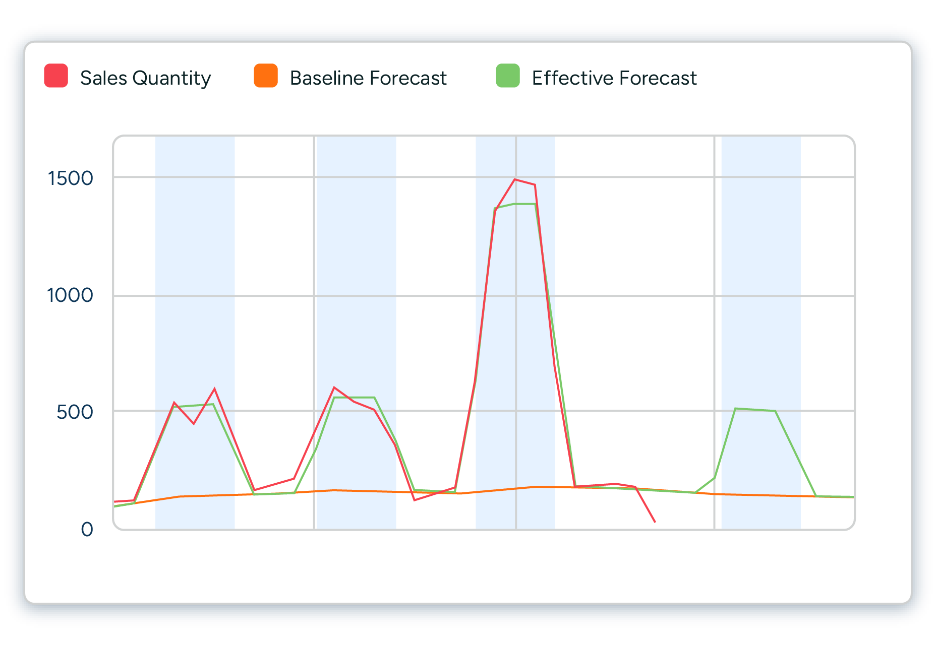
In many cases, it is also very valuable to be able to review what the forecast looked like when an important business decision was made. Was a big purchase order, for example, placed because the actual forecast at that time contained a planned promotion that was later removed? In that case, the root cause for poor forecast accuracy was not the forecasting itself but rather a lack of synchronization in planning.
Measuring forecast accuracy is a good servant but a poor master
You probably see why it’s tempting to create an arbitrary forecast accuracy percentage and move on. However, the focus on improving retail and supply chain planning can easily shift too much towards increasing forecast accuracy at the expense of enhancing the effectiveness of the complete planning process. While our customers enjoy the benefits of increased forecast accuracy with our machine learning algorithms, there is still a need to discuss the role of forecasting in the bigger picture.
For some products, it is easy to attain a very high forecast accuracy. For others, it is more cost-effective to work on mitigating the consequences of forecast errors. For the ones that fall somewhere in between, you need to continuously evaluate the quality of your forecast and how it works with the rest of your planning process. Good forecast accuracy alone does not equate to a successful business.

To summarize, here are the fundamental principles to bear in mind when measuring forecast accuracy:
- First, measure what you need to achieve, such as efficiency or profitability. Use this information to focus on situations where good forecasting matters. Ignore areas where it will make little or no difference. Keep in mind that forecasting is a means to an end. It is a tool to help you get the best results: high sales volumes, low waste, great availability, good profits, and happy customers.
- Understand the role forecasts play in attaining business results and then improve forecasting along with other planning processes. Optimize safety stocks, lead times, planning cycles, and demand forecasting in a coordinated fashion, focusing on the parts of the process that matter the most. Critically review assortments, batch sizes, and promotional activities that do not drive business performance. Great forecast accuracy is no consolation if you are not getting the most important things right.
- Make sure your forecast accuracy metrics match your planning processes and use several metrics in combination. Choose the right aggregation level, weighting, and lag for each purpose and monitor your forecast metrics continuously to spot any changes. Often, the best insights are available when you use more than one metric simultaneously. Most of this monitoring can and should be automated to highlight only relevant exceptions.
- To compare your forecast accuracy with other companies, compare like with like and understand how the formula is calculated. The realistic levels of forecast accuracy can vary significantly from business to business — and even between products in the same segment. The differences in strategy, assortment width, marketing activities, and dependence on external factors like the weather will shift your results. You can easily get significantly better or worse results when calculating essentially the same forecast accuracy metric in different ways. Remember that forecasting is not a competition to get the best numbers. To learn from others, don’t just look at the numbers without context. Instead, study how they approach forecasting and how they use forecasts to develop their planning processes.

Forecast accuracy FAQ
1. Why is forecast accuracy important in demand forecasting?
Demand forecast accuracy helps retailers, wholesalers, and CPG companies make informed inventory management, replenishment, capacity planning, and resource allocation decisions. Accurate demand forecasts reduce uncertainty, improve product availability, minimize spoilage, optimize inventory turnover, and enhance overall supply chain efficiency.
2. How do you determine the quality of a demand forecast?
Two main things can determine the quality of a demand forecast: forecast accuracy and forecast bias. Forecast accuracy is the measure of how accurately a given forecast matches actual sales. Forecast bias describes how much the forecast is consistently over or under the actual sales. Common metrics used to evaluate forecast accuracy include Mean Absolute Percentage Error (MAPE) and Mean Absolute Deviation (MAD). Companies should select the metrics that best align with their business and strategic needs.
3. What is the best way to monitor forecast accuracy?
Monitoring forecast accuracy involves regularly comparing forecasted values with actual values and calculating the relevant accuracy metrics. This process helps identify areas where the forecast may consistently overestimate or underestimate demand, allowing for adjustments and improvements. It’s essential to track forecast accuracy over time and across different levels of granularity to ensure the forecasting process remains effective and aligned with business objectives. Ensure to measure forecast accuracy where it truly impacts products and situations, or your efforts will be wasted.
